← [Documentation index](README.md)
# Frequency Weighting (A, C, G, Z)
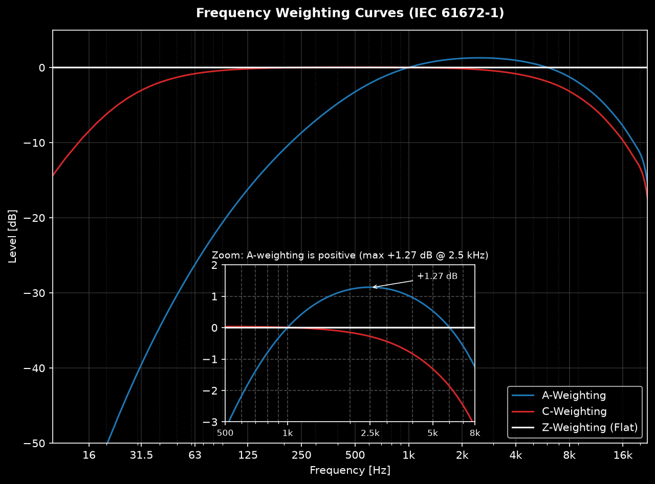
Frequency weighting curves simulate the human ear's sensitivity. A, C and Z
are specified by **IEC 61672-1:2013**; the infrasound G curve is specified by
**ISO 7196:1995**.
* **A-Weighting (`A`):** Standard for environmental noise (IEC 61672-1).
* **C-Weighting (`C`):** Used for peak sound pressure and high-level noise.
* **Z-Weighting (`Z`):** Zero weighting, completely flat response.
* **G-Weighting (`G`):** Infrasound weighting per ISO 7196 (see below).
```python
from phonometry import weighting_filter
# Apply A-weighting to the raw signal
weighted_signal = weighting_filter(signal, fs, curve='A')
# Apply C-weighting for peak analysis
c_weighted_signal = weighting_filter(signal, fs, curve='C')
```
## Infrasound: G-weighting (ISO 7196)
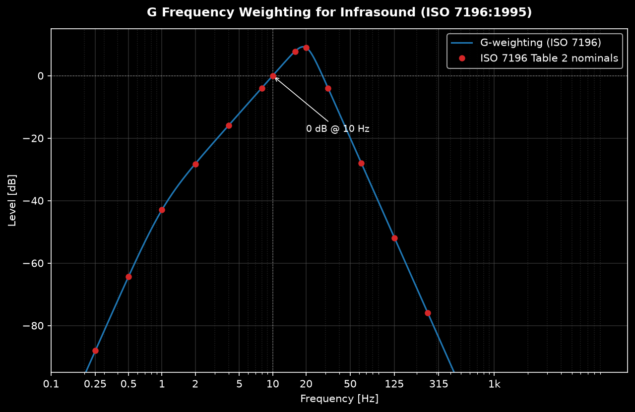
The **G frequency weighting** (ISO 7196:1995) rates infrasound the way A-weighting
rates audible noise. It is defined by a pole-zero configuration with 0 dB gain at
10 Hz, rises at 12 dB/octave from 1 Hz to 20 Hz (matching the steep growth of
perception in that band) and falls off at 24 dB/octave outside it. Use it for
sources with significant energy below 20 Hz (wind turbines, HVAC, blasting):
```python
from phonometry import weighting_filter
g_weighted = weighting_filter(signal, fs, curve='G')
```
The implementation follows the ISO 7196 Table 1 pole/zero values exactly and is
verified in CI against every Table 2 nominal response value (0.25 Hz to 315 Hz).
`WeightingFilter(fs, "G")` supports the same multichannel and stateful block
processing as A/C. Levels measured with the G curve are reported as
LpG (or LGeq for the equivalent level over time).
## Where the curves come from
The A and C curves are inverted equal-loudness contours, frozen into filters:
**A** approximates the inverse of the historic 40-phon contour (quiet levels,
where the ear discards bass most aggressively) and **C** the flatter ~100-phon
one (loud levels). IEC 61672-1:2013 (Annex E) defines both analytically from
four corner frequencies:
$$
f_1 = 20.599\ \text{Hz}, \quad f_2 = 107.653\ \text{Hz}, \quad
f_3 = 737.862\ \text{Hz}, \quad f_4 = 12194.217\ \text{Hz}
$$
C is a band-pass with double poles at $f_1$ and $f_4$ (2 zeros at the origin);
A adds the $f_2$ and $f_3$ poles (4 zeros), which is why it keeps falling
through the low-mids. Both are normalized to exactly 0 dB at 1 kHz. Z is the
absence of weighting. The full pole/zero derivation is in the
[Theory](theory.md) page.
### `weighting_filter()` / `WeightingFilter` parameters
| Parameter | Type | Units | Range / default | Notes |
| :--- | :--- | :--- | :--- | :--- |
| `x` | 1D or 2D array | any | non-empty | 2D is `[channels, samples]` |
| `fs` | int | Hz | > 0 | |
| `curve` | str | — | `'A'` (default), `'C'`, `'G'`, `'Z'` | `'G'` per ISO 7196 (infrasound); `'Z'` is a bypass |
| `high_accuracy` | bool | — | default `True` (function); class default `None` resolves to `not stateful` | Internal oversampling (8× up to ≥ 96 kHz at common audio rates) keeps A/C in class 1 up to 16 kHz; silently ignored for G, whose 0.25–315 Hz range the plain design already renders exactly |
| `stateful` | bool (class only) | — | default `False` | Carries filter state across blocks (streaming) |
| `steady_ic` | bool (class only) | — | default `False` | Steady-state initial conditions (no onset transient) |
## Reusable filter object
If you weight many signals with the same parameters, design the filter once:
```python
from phonometry import WeightingFilter
wf = WeightingFilter(fs, "A")
for signal in signals:
weighted = wf.filter(signal)
```
## High-frequency accuracy (`high_accuracy`)
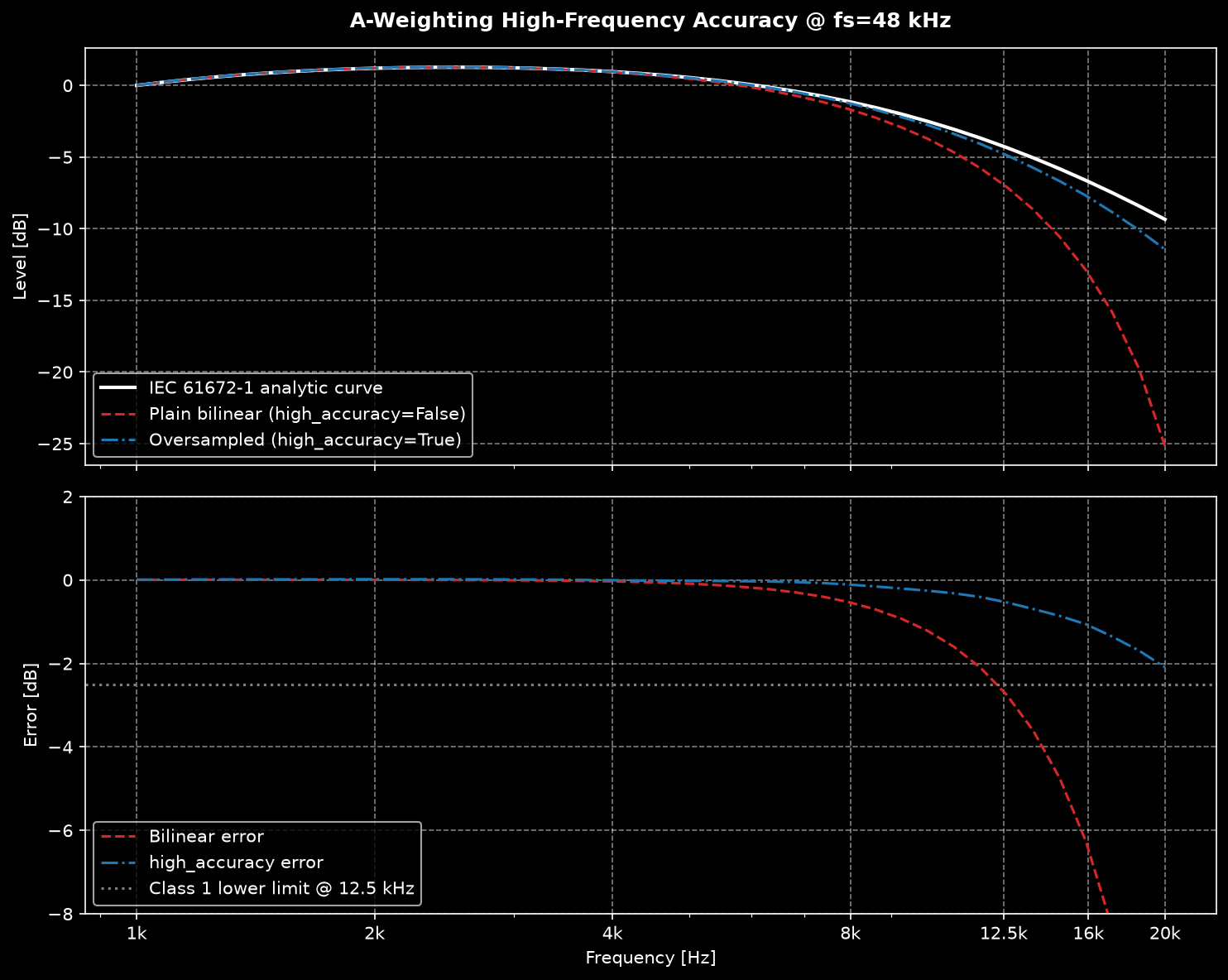
A plain bilinear-transform design compresses the response near Nyquist: at
fs = 48 kHz the A-curve error at 12.5 kHz reaches −2.7 dB, outside the IEC
61672-1 **class 1** tolerance (+2.0/−2.5 dB).
By default (`high_accuracy=True`), phonometry designs and runs the weighting
filter at an internally oversampled rate (≥ 96 kHz) and decimates back, keeping
the response within class 1 tolerances up to 16 kHz (error ≈ −0.5 dB at
12.5 kHz for fs = 48 kHz).
*The plain bilinear design (red) crosses the class 1 tolerance near 12.5 kHz;
the oversampled design (blue) stays close to the analytic curve.*
- `high_accuracy=False` restores the legacy plain-bilinear behavior.
- **Stateful (block) processing** always uses the legacy design: the internal
FIR resampling is incompatible with block continuity. Passing
`high_accuracy=True` together with `stateful=True` raises a `ValueError`.
```python
# Explicit legacy behavior
y = weighting_filter(signal, fs, curve="A", high_accuracy=False)
# Stateful block processing (legacy design, state carried between blocks)
wf = WeightingFilter(fs, "A", stateful=True)
for block in blocks:
weighted = wf.filter(block)
```
See [Block Processing](block-processing.md) for the streaming workflow and
[Theory](theory.md) for the analytic curve definitions.