← [Documentation index](README.md)
# Integrated and Statistical Levels
Environmental noise metrics computed directly from the raw (calibrated) signal.
## Leq and LAeq
The equivalent continuous level integrates the squared pressure over the
measurement time:
$$
L_{eq} = 10\log_{10}\left(\frac{1}{T}\int_0^T \frac{p^2(t)}{p_0^2}\ dt\right) \text{ dB}, \qquad p_0 = 20\ \mu\text{Pa}
$$
and $L_{Aeq}$ is the same integral after A-weighting the signal. $L_N$ is the
level exceeded $N\ \%$ of the time — the $(100-N)$-th percentile of the
time-weighted level distribution.
```python
import numpy as np
from phonometry import leq, laeq
# recording: a calibrated microphone capture (Pa) — recorded through your measurement chain. Synthesized here so the guide runs standalone.
fs = 48000
recording = 0.2 * np.sin(2 * np.pi * 1000 * np.arange(fs) / fs)
sensitivity = 1.0 # calibration_factor (see Calibration)
# Equivalent continuous level of the whole recording
level = leq(recording, calibration_factor=sensitivity)
# A-weighted Leq (the standard environmental noise metric)
la = laeq(recording, fs, calibration_factor=sensitivity)
```
Both accept 1D signals (returning a scalar) or 2D `[channels, samples]` arrays
(returning one level per channel), and support `dbfs=True` for digital
full-scale analysis (calibration does not apply in dBFS mode).
Why the *energy* mean and not the arithmetic mean of dB values? Because sound
doses add as energy: two periods at 60 dB and 80 dB do not average to 70 dB —
the 80 dB half dominates and $L_{eq}$ = 77 dB. Averaging decibels directly
underestimates every fluctuating noise. $L_{eq}$ is the level of the *steady*
sound carrying the same energy as the real, fluctuating one, which is why
regulations are written in terms of it.
### `leq()` / `laeq()` parameters
| Parameter | Type / shape | Units | Range / default | Notes |
| :--- | :--- | :--- | :--- | :--- |
| `x` | 1D or 2D array | digital units (or Pa if calibrated) | non-empty | 2D is `[channels, samples]`; returns one level per channel |
| `fs` | int | Hz | > 0 (`laeq` only) | `leq` needs no sample rate (pure RMS integral) |
| `calibration_factor` | float | Pa per digital unit | default `1.0` | From `calculate_sensitivity()` |
| `dbfs` | bool | — | default `False` | `True`: 0 dBFS = full-scale RMS sine; ignores calibration |
## Percentile levels (LN)
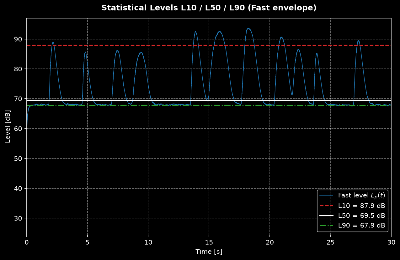
`ln_levels` computes statistical levels from the time-weighted envelope:
**L10** is the level exceeded 10 % of the time (event peaks), **L50** the median,
**L90** the background level.
```python
from phonometry import ln_levels
# A steady tone gives L10 = L50 = L90; percentiles only tell a story for a
# *fluctuating* level. Synthesize 3 s alternating between a quiet and a
# ~10 dB louder half-second so the statistics separate.
rng = np.random.default_rng(0)
segment = fs // 2 # 0.5 s per level
quiet = 0.02 * rng.standard_normal(segment) # background
loud = 0.06 * rng.standard_normal(segment) # ~10 dB louder events
varying = np.tile(np.concatenate([quiet, loud]), 3)
stats = ln_levels(varying, fs, n=(10, 50, 90), weighting="A")
print(f"LA10={stats[10]:.1f} LA50={stats[50]:.1f} LA90={stats[90]:.1f} dB")
# LA10=66.6 LA50=65.2 LA90=58.5 dB -> L10 (events) > L50 (median) > L90 (background)
```
*L10 tracks the event peaks, L50 the median level and L90 the background.*
Options: `mode` selects the envelope ballistics (`'fast'`, `'slow'`,
`'impulse'`), `weighting` applies A/C weighting first, and
`calibration_factor`/`dbfs` behave as in `leq`. The integrator attack transient
(~5τ) is discarded before taking percentiles, so the leading settling ramp is
not counted in the low percentiles.
Formally, $L_N$ is the $(100-N)$-th percentile of the distribution of the
time-weighted level: the recording is first turned into a level-vs-time
envelope (Fast by default), and $L_{10}$ is the envelope value exceeded 10 %
of the time. That makes the *ballistics choice part of the metric*: an
$L_{10}$ from a Slow envelope is systematically lower than from a Fast one on
impulsive noise, so regulations always name the time weighting.
### `ln_levels()` parameters
| Parameter | Type / shape | Units | Range / default | Notes |
| :--- | :--- | :--- | :--- | :--- |
| `x` | 1D or 2D array | digital units | non-empty | 2D returns per-channel dicts |
| `fs` | int | Hz | > 0 | Needed by the envelope detector |
| `n` | tuple of ints | % | default `(10, 50, 90)` | Any exceedance percentages, e.g. `(1, 5, 95)` |
| `mode` | str | — | `'fast'` (default), `'slow'`, `'impulse'` | IEC 61672-1 ballistics of the envelope |
| `weighting` | str or None | — | `'A'`, `'C'`, `'G'`, `'Z'`, `None` (default) | Frequency weighting before the envelope |
| `calibration_factor` / `dbfs` | float / bool | — | as `leq` | Same semantics as in `leq()` |
## Peak, event and occupational metrics
```python
from phonometry import lc_peak, sel, sound_exposure, lex_8h
# C-weighted peak (IEC 61672-1 §5.13) - occupational action limits use this
peak = lc_peak(recording, fs, calibration_factor=sensitivity)
# A single noise event and a work-shift sample (slices of a real recording)
event = recording
shift_sample = recording
# Sound exposure level: single-event level normalized to 1 s (LAE)
lae = sel(event, fs, weighting="A", calibration_factor=sensitivity)
# Daily noise dose (IEC 61252): exposure in Pa²·h and LEX,8h / LEP,d
E = sound_exposure(shift_sample, fs, duration_hours=8, calibration_factor=sensitivity)
lex = lex_8h(shift_sample, fs, duration_hours=8, calibration_factor=sensitivity)
```
`lc_peak` is verified against the one-cycle/half-cycle reference responses of
IEC 61672-1:2013 Table 5, `sel` against the Table 4 LAE toneburst column, and
the dose functions against the IEC 61252 anchors (3.2 Pa²h ↔ exactly 90 dB).
`lc_peak` polyphase-oversamples the C-weighted signal by `oversample` (default
`8`) before taking the maximum, recovering the true inter-sample peak: a raw
on-grid maximum under-reads sustained HF tones by up to ~1.15 dB (an 8 kHz tone
at 48 kHz is only 6 samples/cycle). Set `oversample=1` to detect the peak on the
original sample grid. With `duration_hours`, the input is treated as a
representative sample of that exposure period; without it, the input is the
whole event.
### SEL: comparing events of different duration
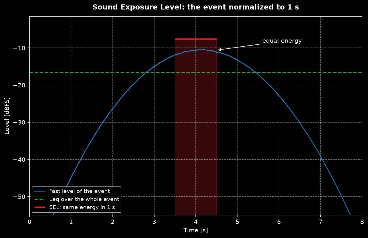
A 4 s train pass-by and a 30 s one cannot be compared by their $L_{Aeq}$
alone — the longer event delivers more energy at the same level. The **sound
exposure level** compresses the *whole* event energy into exactly one second:
$$
L_E = L_{eq,T} + 10\log_{10}\frac{T}{T_0}, \qquad T_0 = 1\ \text{s}
$$
so events of any duration become directly comparable, and $N$ identical
events sum as $+10\log_{10}N$. This is the building block of airport and
railway noise models.
### Noise dose: sound exposure and LEX,8h
Occupational regulations limit the daily *dose*, not the level. IEC 61252
expresses it as **sound exposure** $E$ in pascal-squared-hours — the time
integral of the squared A-weighted pressure — and the equivalent
**normalized 8 h level**:
$$
E = \int_0^T p_A^2(t)\ dt \quad [\text{Pa}^2\text{h}], \qquad
L_{EX,8h} = 10\log_{10}\frac{E}{8\ \text{h} \cdot p_0^2}
$$
The anchor worth memorizing: **3.2 Pa²h ⇔ exactly 90 dB over 8 h** (the CI
suite enforces it). Half the dose is −3 dB; double duration at the same level
is +3 dB.
### Peak / event / dose parameters
| Function | Key parameters | Returns | Standard anchor |
| :--- | :--- | :--- | :--- |
| `lc_peak(x, fs, calibration_factor=1.0, dbfs=False)` | `dbfs=True` references full-scale *peak* (1.0), not RMS | LCpeak [dB] | IEC 61672-1 §5.13, Table 5 tone bursts |
| `sel(x, fs, weighting=None, ...)` | `weighting='A'` gives LAE | SEL [dB] | IEC 61672-1 Table 4 (LAE column) |
| `sound_exposure(x, fs, duration_hours=None, ...)` | `duration_hours` treats `x` as a sample of that period | E [Pa²h] | IEC 61252 |
| `lex_8h(x, fs, duration_hours=None, ...)` | same sampling semantics | LEX,8h [dB] | IEC 61252 (≡ LEP,d) |
## Occupational noise exposure strategies and uncertainty (ISO 9612)
`lex_8h` above turns *one* recording into a daily level. ISO 9612:2009 — the
engineering method (accuracy grade 2) — is the survey design *around* that
primitive: how to sample a real working day, how to combine the pieces, and how
to attach the normative uncertainty every occupational-hygiene report needs. The
`occupational_exposure` module adds the three **measurement strategies** and the
**Annex C** uncertainty budget on top of the energy-average machinery.
The *task-based* strategy (Clause 9) splits the nominal day into tasks, takes
$I \ge 3$ samples per task, and energy-sums the task contributions
$$
L_{EX,8h,m} = L_{p,A,eqT,m} + 10 \log_{10}(T_m/T_0), \qquad T_0 = 8\ \text{h},
$$
so a loud but short task contributes little. The *job-based* (Clause 10) and
*full-day* (Clause 11) strategies instead take $N \ge 5$ (or three whole-day)
random samples over a homogeneous exposure group and normalise the effective-day
duration. The daily level is the same either way; the strategies differ in how
the **uncertainty** is built.
```python
from phonometry.occupational_exposure import (
Task, task_based_exposure, job_based_exposure, full_day_exposure,
)
# ISO 9612 Annex D — a welder's day split into three tasks. Each task level is
# the energy average of its Lp,A,eqT samples; durations carry a measured range.
tasks = [
Task(samples=(70.0,), duration_hours=1.5, label="planning/breaks"),
Task(samples=(80.1, 82.2, 79.6), duration_hours=5.0,
duration_range=(4.0, 6.0), label="welding"),
Task(samples=(86.5, 92.4, 89.3, 93.2, 87.8, 86.2), duration_hours=1.5,
duration_range=(1.0, 2.0), label="cutting/grinding"),
]
res = task_based_exposure(tasks, include_duration_uncertainty=False, warn=False)
print(f"LEX,8h = {res.lex_8h:.1f} dB U = {res.expanded_uncertainty:.1f} dB")
# LEX,8h = 84.3 dB U = 2.7 dB
print(f"one-sided 95 % upper limit LEX,8h + U = {res.upper_limit:.1f} dB") # 87.0 dB
for t in res.tasks:
print(f" {t.label:<16} Lp,A,eqT = {t.lp_aeqt:5.1f} contributes {t.lex_8h_contribution:5.1f} dB")
# planning/breaks Lp,A,eqT = 70.0 contributes 62.7 dB
# welding Lp,A,eqT = 80.8 contributes 78.7 dB
# cutting/grinding Lp,A,eqT = 90.1 contributes 82.8 dB
# The same shift measured job-based (Annex E) and full-day (Annex F): both use
# the Eq C.9 / Table C.4 sampling budget with k = 1.65 (one-sided 95 %).
job = job_based_exposure([88.1, 86.1, 89.7, 86.5, 91.1, 86.7], effective_duration_hours=7.5)
full = full_day_exposure([88.0, 91.9, 87.6, 90.4, 89.0, 88.4], effective_duration_hours=9.25)
print(f"job LEX,8h = {job.lex_8h:.1f} dB U = {job.expanded_uncertainty:.1f} dB")
# job LEX,8h = 88.2 dB U = 3.8 dB
print(f"full-day LEX,8h = {full.lex_8h:.1f} dB U = {full.expanded_uncertainty:.1f} dB")
# full-day LEX,8h = 90.1 dB U = 3.4 dB
```
Two subtleties are worth spelling out. First, the coverage factor is
$k = 1.65$ for a **one-sided** 95 % interval (Clause 14), because a hygienist
cares only about the *upper* bound: `res.upper_limit` = $L_{EX,8h} + U$ is the
value 95 % of measurements fall below, the number compared against an action
limit. Second, the task and job methods weight the *same* spread of samples
differently. The task sampling uncertainty $u_{1a}$ (Eq. C.6) divides the summed
squared deviations by $I(I-1)$ — the standard error of the mean, smaller by a
factor $\sqrt{I}$ — whereas the job/full-day sampling uncertainty $u_1$ (Eq. C.12)
is the plain sample standard deviation with denominator $N-1$, whose contribution
$c_1 u_1$ is then read from **Table C.4** as a function of $(N, u_1)$. The same
raw scatter therefore inflates the job estimate more, which is the standard's
built-in penalty for coarser, fewer samples. (The printed job $L_{EX,8h}$ is
$88.2$ dB where Annex E reports $88.1$: the standard rounds the effective-day
level to $88.4$ before the duration normalisation; the library keeps it
unrounded.)
When a task's samples span **3 dB or more** (Clause 9.3), or the job contribution
$c_1 u_1$ exceeds 3.5 dB (Clause 10.4), or too few workers are covered
(Table 1 cumulative-duration), the result sets `sampling_advisory=True` and, with
`warn=True`, emits an `ExposureWarning` recommending more measurements. Peak
levels $L_{p,Cpeak}$ are reported **without** an uncertainty — Annex C gives no
method for them (Table C.5, Note 1), so peak-uncertainty is out of scope. The
three Annex D/E/F worked examples above are reproduced to the standard's printed
precision (Annex E's final rounding is disclosed above), and the theory is
derived on the [Theory](theory.md) page.
### `task_based_exposure()` / `job_based_exposure()` / `full_day_exposure()` parameters
| Parameter | Applies to | Type | Units | Range / default | Notes |
| :--- | :--- | :--- | :--- | :--- | :--- |
| `tasks` | task | list of `Task` | — | ≥ 1 | Each `Task` has `samples`, `duration_hours`, optional `duration_range`/`duration_samples`, `label`, `instrument` |
| `samples` | job / full-day | sequence | dB | ≥ 2 (≥ 5 / ≥ 3 advised) | Random `Lp,A,eqT` samples |
| `effective_duration_hours` | job / full-day | float | h | > 0 | Effective working-day duration $T_e$ |
| `instrument` | all | str | — | `'class1'`, `'class2'`, `'personal_exposimeter'` (default) | Selects $u_2$ (Table C.5) |
| `u3` | all | float | dB | default `1.0` | Microphone-position uncertainty (Clause C.6) |
| `include_duration_uncertainty` | task | bool | — | default `True` | `False` omits the $(c_{1b}u_{1b})^2$ term (Annex D case a) |
| `n_workers` / `sample_duration_hours` | job | int / float | — / h | default `None` | Table 1 cumulative-duration check |
| `warn` | all | bool | — | default `True` | Emit `ExposureWarning` for the sampling advisories |
All three return an `ExposureResult` with `lex_8h`, `combined_standard_uncertainty`
$u$, `expanded_uncertainty` $U = 1.65\ u$, `upper_limit` = $L_{EX,8h} + U$,
`sampling_advisory`, and (task-based) the per-task `tasks` breakdown.
## Loudness level of pure tones (ISO 226:2023)
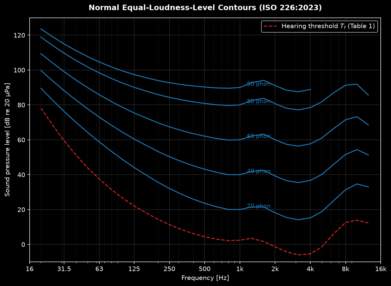
The normal equal-loudness-level contours relate the SPL of a pure tone to its
perceived *loudness level* in phons (the SPL of an equally loud 1 kHz tone).
`equal_loudness_contour(phon)` evaluates ISO 226:2023 Formula (1) at the 29
preferred third-octave frequencies of Table 1, `loudness_level(spl, frequency)`
is the exact inverse (Formula 2), and `hearing_threshold()` returns the
threshold-of-hearing column:
```python
from phonometry import equal_loudness_contour, loudness_level
freqs, spl = equal_loudness_contour(40.0) # the classic 40-phon contour
phon = loudness_level(73.0, 63.0) # 73 dB @ 63 Hz -> 40 phon
```
Validity per clause 4.1: 20-90 phon (80 phon above 4 kHz); the implementation
is verified against the Annex B tables in CI. Note this is the loudness of
*pure tones* - loudness of arbitrary signals (ISO 532 sones) is a different,
upcoming feature.
## Prominent discrete tones (ECMA-418-1)
Tonal components in machinery noise are far more annoying than their level
suggests. ECMA-418-1:2024 (referenced by ECMA-74 Annex D) gives two FFT-based
methods to decide whether a discrete tone is *prominent*:
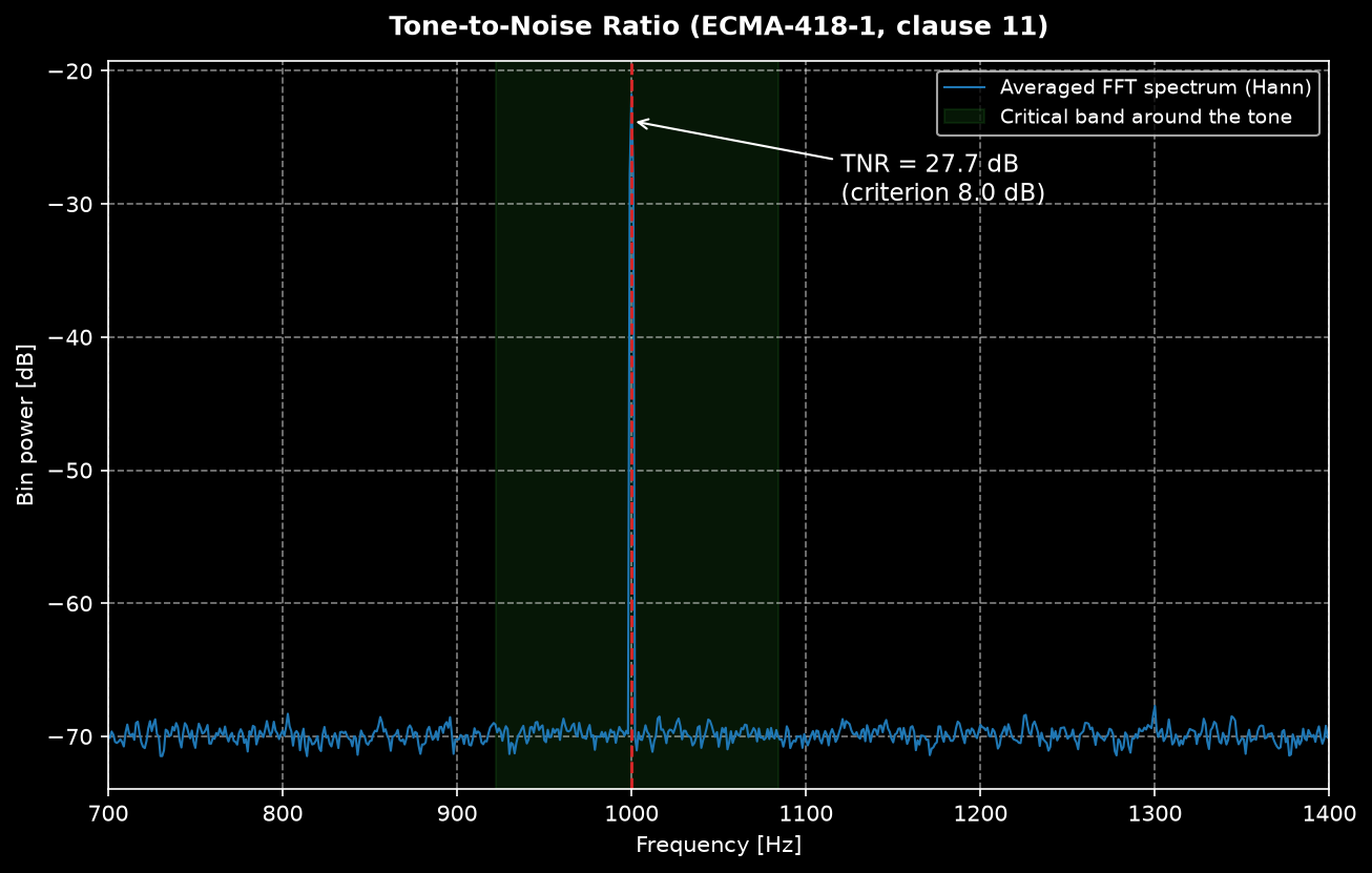
`tone_to_noise_ratio()` compares the tone level with the masking noise in its
critical band (clause 11), and `prominence_ratio()` compares the critical band
centred on the tone with the two contiguous bands (clause 12). Both return a
structured verdict against the frequency-dependent prominence criteria:
```python
import numpy as np
from phonometry import tone_to_noise_ratio, prominence_ratio
fs = 48000
rng = np.random.default_rng(0)
t = np.arange(fs) / fs
x = np.sin(2 * np.pi * 1000 * t) + 0.05 * rng.standard_normal(fs) # 1 kHz tone in noise
tnr = tone_to_noise_ratio(x, fs) # highest peak, or tone_freq=...
pr = prominence_ratio(x, fs, tone_freq=1000.0)
print(tnr.ratio_db, tnr.criterion_db, tnr.prominent)
```
The methods hinge on the **critical band** — the ear's analysis bandwidth,
$\Delta f_c = 25 + 75\ [1 + 1.4(f/1000)^2]^{0.69}$ Hz (162 Hz at 1 kHz): a
tone is masked only by the noise *inside* its critical band, so both ratios
compare the tone against exactly that noise, not the whole spectrum.
A TNR above $8 + 8.33\log_{10}(1000/f_t)$ dB (8 dB from 1 kHz up) classifies
the tone as *prominent*; the PR criterion is $9 + 10\log_{10}(1000/f_t)$ dB.
Low frequencies get higher thresholds because wider relative bands mask more.
ECMA-74 (which delegates its tone assessments to ECMA-418-1) also fixes where to measure around a device:
Proximate secondary tones in the same critical band are combined per
clause 11.6; for harmonic complexes assess each component (`tone_freq=`).
Both methods work on Hann-windowed, RMS-averaged spectra and need no absolute
calibration (the ratios are level differences).
### `tone_to_noise_ratio()` / `prominence_ratio()` parameters
| Parameter | Type | Units | Range / default | Notes |
| :--- | :--- | :--- | :--- | :--- |
| `x` | 1D array | any (uncalibrated OK) | ≥ `fs/resolution_hz` samples | Ratios are level differences: calibration cancels out |
| `fs` | int | Hz | > 0 | |
| `tone_freq` | float, optional | Hz | 89.1–11 200; default `None` | `None` assesses the highest peak in the range of interest |
| `resolution_hz` | float | Hz | > 0; default `1.0` | Tone band must stay within 15 % of the critical band (clause 11.2) |
Both return a `ToneAssessment(frequency, ratio_db, criterion_db, prominent)`.
## Environmental noise: Lden, Ldn and rating levels (ISO 1996-1)
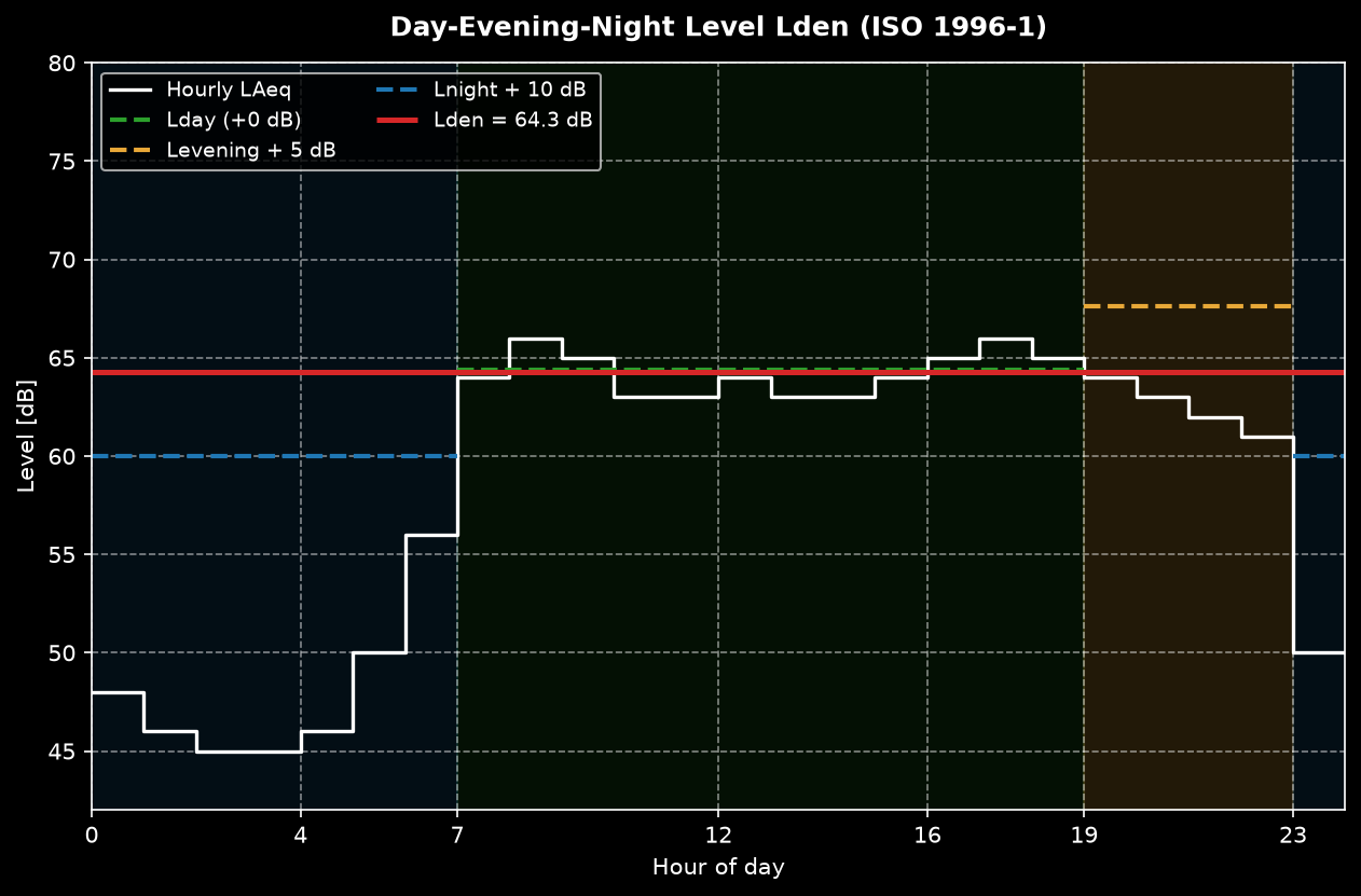
Regulatory noise assessment weights evenings and nights more heavily.
`lden()` implements the day-evening-night level of ISO 1996-1:2016 (3.6.4:
+5 dB evening, +10 dB night, default 12/4/8 h periods — adjustable, since
countries define them differently), `ldn()` the day-night variant (3.6.5),
and `composite_rating_level()` the general whole-day composite of clause 6.5
(Formulae 5-6) for arbitrary periods with source or character adjustments
(Table A.1: e.g. +5 dB regular impulsive, +12 dB highly impulsive, +3 to
+6 dB prominent tones):
```python
from phonometry import lden, composite_rating_level
l = lden(63.2, 58.1, 51.4) # from LAeq per period
r = composite_rating_level([(63.2, 12, 0.0), # day
(58.1, 4, 5.0), # evening (+5)
(51.4, 8, 10.0)]) # night (+10) == lden
```
### `lden()` / `ldn()` / `composite_rating_level()` parameters
| Function | Key parameters | Notes |
| :--- | :--- | :--- |
| `lden(lday, levening, lnight, hours=(12, 4, 8))` | period LAeq values [dB]; `hours` must sum to 24 | +5 dB evening, +10 dB night (3.6.4) |
| `ldn(lday, lnight, hours=(15, 9))` | | +10 dB night (3.6.5) |
| `composite_rating_level(periods)` | iterable of `(level_db, hours, adjustment_db)`; hours positive, finite and summing to 24 | General Formulae (5)-(6); adjustments per Table A.1 |
Where you put the microphone changes the number: ISO 1996-2 fixes the receiver positions and their façade corrections:
Combine with `laeq()` per time period to go from recordings to Lden, and with
`tone_to_noise_ratio()` / `prominence_ratio()` to justify tonal adjustments.
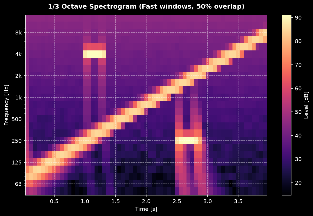
## Octave Spectrogram (levels over time)
Short-time fractional-octave analysis: one level per band per window,
time-aligned across bands.
```python
from phonometry import OctaveFilterBank
bank = OctaveFilterBank(fs=48000, fraction=3)
levels, freq, times = bank.spectrogram(recording, window_time=0.125, overlap=0.5)
# levels: (bands, frames) — ready for pcolormesh(times, freq, levels)
```
*A logarithmic sweep plus two tone bursts, resolved in time and in standardized
1/3-octave bands.*
- Multichannel input `(channels, samples)` returns `(channels, bands, frames)`.
- `times` holds each window's center in seconds.
- `mode='peak'` gives per-window peak-holding levels instead of RMS.
- `zero_phase=True` filters bands forward-backward so per-band group delay does
not skew the frames (offline analysis only).
### `OctaveFilterBank.spectrogram()` parameters
| Parameter | Type | Units | Range / default | Notes |
| :--- | :--- | :--- | :--- | :--- |
| `x` | 1D or 2D array | digital units | non-empty | 2D returns `(channels, bands, frames)` |
| `window_time` | float | s | > 0; default `0.125` | Frame length (0.125 s mirrors Fast) |
| `overlap` | float | — | 0 ≤ overlap < 1; default `0.5` | Fraction of window overlap (0 = none) |
| `mode` | str | — | `'rms'` (default) or `'peak'` | Per-window detector |
| `detrend` | bool | — | default `True` | Remove each band's DC offset before the level (improves low-frequency accuracy) |
| `zero_phase` | bool | — | default `False` | Forward-backward filtering (offline only) |
| `calibration_factor` / `dbfs` | — | — | constructor-only | Set on `OctaveFilterBank(...)`, not per call |
```python
import matplotlib.pyplot as plt
fig, ax = plt.subplots()
mesh = ax.pcolormesh(times, freq, levels, shading="auto")
ax.set_yscale("log")
ax.set_xlabel("Time [s]")
ax.set_ylabel("Frequency [Hz]")
fig.colorbar(mesh, label="Level [dB]")
```
See [Calibration and dBFS](calibration.md) to convert digital units to physical
SPL, and [Time Weighting](time-weighting.md) for the envelope details.